Introduction to Air Quality Modeling: Ozone Modeling Procedure
This page describes the general air quality modeling procedure for developing State Implementation Plans for ozone nonattaiment areas in Texas.
1. Modeling Protocol
For modeling used to support Attainment Demonstration SIP revisions, a Modeling Protocol is required by EPA (see Modeling Guidance for Demonstrating Attainment of Air Quality Goals for Ozone, PM2.5, and Regional Haze ). The Protocol includes plans for:
- Specification of policy and technical review groups
- Definition of modeling domains
- Periods to be modeled (episodes)
- Meteorological modeling
- Base-and future-case emissions modeling
- Specification of the photochemical modeling platform
- Base-case model performance evaluation
- Future-case modeling
2. Base-Case Modeling — Reproducing the Past
Modeling for attainment demonstration SIP revisions uses selected periods from recent years, which are referred to as episodes. The episodes are typically months to seasons long and include days where high concentrations of ozone were measured in the area of interest. The area of interest (nonattainment area) is surrounded by three-dimensional gridded boxes called domains, with the finest resolution near the area of interest.
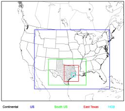
Example of Nested Modeling Domains
Once the period to be modeled and modeling domains are selected, meteorological modeling is conducted for the entire period to provide a three-dimensional characterization of the atmosphere, including important parameters like wind, temperature, and solar radiation for each hour and in every location in the domain.
Simultaneously, emissions from all sources (vehicles, industry, construction, vegetation, ships, etc.) are modeled across the entire modeling domain for each hour. The emissions and meteorology are input into the photochemical model to simulate the base-case modeled pollutant concentrations.
By comparing the base case photochemical model's results to observations of ozone, nitrogen oxides, and volatile organic compounds concentrations, the confidence in the model's ability is determined. Also, modeled concentrations of important chemicals that are emitted, created, or destroyed in the model's chemical and physical processes are compared with available measurements. This performance evaluation helps determine that the model “gets the right answer for the right reason.”
3. Future-Year Modeling — Predicting the Future
Once satisfactory model performance has been achieved for the base case, econometric forecasts are used to estimate the growth of emissions from industry, traffic, and population to each area’s attainment year (future year) as established by the federal Clean Air Act (CAA). These estimates are then adjusted to account for “on-the-books” federal, state, and local regulations.
Predicted future year emissions are then substituted into the base case model (the meteorology is left unchanged) to create the future-case model. The future case model is run and predicted future pollutant concentrations are compared to base case concentrations to find the model’s response to predicted growth and regulations. If the model's response shows predicted ozone concentrations are below the federal limit at every regulatory monitor, then the model provides strong evidence that attainment will be reached in the future year modeled.
4. Modeling Emissions Controls for the SIP
If the existing regulations are not sufficient, the TCEQ works with stakeholders to find strategies that reduce emissions enough to achieve attainment. The model is used to evaluate the effectiveness of these strategies and to provide evidence that attainment will be reached once a strategy has been chosen.
In addition to the modeling, the attainment demonstration revision includes additional analyses designed to challenge the conclusion that attainment will be reached. These analyses may include trend analyses, third-party photochemical modeling, other types of modeling analyses, and anything else that provides evidence as to whether or not attainment will be reached. These analyses are weighed together with the conclusions of the modeling, and if the balance of evidence supports the conclusion that attainment will be reached, an attainment demonstration SIP revision is prepared, reviewed, presented for public comment, and delivered to EPA.